Definition of graph

A graph is a data structure composed of a vertex set V and a relationship set E (a set of edges) between vertices. It can be defined as a tuple: G = (V, E)

basic terminology

1. Directed and undirected graphs

   In a graph, if the edges have direction, it is called a directed graph; if the edges have no direction, it is called an undirected graph.

2. Complete graph, dense graph, sparse graph

   • A graph with n vertices and n(n-1)/2 edges is called a completely undirected graph.
   • A directed graph with n vertices and n(n-1) arcs is called a complete directed graph.
   • Completely undirected graphs and completely directed graphs are both called complete graphs.
   • For a general undirected graph, the number of vertices is n and the number of edges is e, then 0<=e<=n(n-1)/2
   • For a general directed graph, the number of vertices is n and the number of arcs is e, then 0<=e<=n(n-1)
   • When a graph is close to a complete graph, it is called a dense graph. On the contrary, when a graph contains fewer edges or arcs, it is called a sparse graph.

3. Degree, in-degree, out-degree

   • In a graph, the number of edges or arcs attached to a vertex is called the degree of the vertex.
   • In a directed graph, the number of arc heads attached to a vertex is called the in-degree of the vertex, the number of arc tails attached to a vertex is called the out-degree of the vertex, and the sum of the in-degree and out-degree of a vertex is called the degree of the vertex.

Graph storage

The storage structure of graphs can be divided into 5 types:

1. adjacency matrix

   The adjacency matrix storage method of a graph is to use two arrays to represent the graph:

   A one-dimensional array stores vertex information in the graph; (vertex array)
   A two-dimensional array (called an adjacency matrix) stores information about edges or arcs in a graph (edge array)

2. adjacency list

   The adjacency matrix is a good graph storage structure.However: For graphs with fewer edge trees than vertices, this structure is a huge waste of storage space.

   Therefore, consider using adjacency list storage.

3. cross linked list

   • For directed graphs, adjacency lists are also flawed.
   • Just think about it, if you care about the out-degree problem, if you want to understand the in-degree problem, you have to traverse the entire graph to know it.
   • On the contrary, the inverse adjacency list solves the in-degree problem but does not understand the out-degree problem.
   • Is it possible to combine adjacency lists and inverse adjacency lists?The answer is yes.
   • This is the so-called storage structure: Cross linked list.

4. adjacency multiple list

   • The optimized storage structure of a directed graph is a cross-linked list.
   • For the adjacency list of an undirected graph, when deleting an edge, two corresponding edge nodes need to be found and processed.
   • This operation is more troublesome, and adjacency multiple tables can improve this problem.

5. edge set array

   • The edge set array focuses on operations that process edges in sequence, and is not suitable for operations related to vertices.
   • The edge set array consists of two one-dimensional arrays, one stores vertex information and the other stores edge information, including starting point subscript (start), end point subscript (end) and weight (weight)

   Graph traversal

Two graph traversal algorithms:

1. Depth first traversal (Depth_First_Search), also known as depth first search, referred to as DFS
2. Breadth first traversal (Breadth_First_Search), also known as breadth first search, referred to as BFS.

Depth-first traversal is similar to pre-order traversal of a tree, and breadth-first traversal is similar to level-order traversal of a tree.

depth first search

The idea behind depth-first search 🔖 : Similar to preorder traversal of a tree (around the root)

1. First visit vertex i and set its access mark to visited, that is, visited[i]=1;
2. Then check the vertex j adjacent to vertex i.If j has not been visited, visit it, set visited[j]=1, and repeat the process starting from j; if j has been visited, continue to check other adjacent vertices of i.
3. If all vertices connected to i have been visited, return to the previously visited vertex and repeat the process until all vertices reachable from the starting point have been visited.If there are still unvisited vertices in the graph, choose another starting point to continue traversing.

breadth first search

The idea used in breadth-first search🔖: Queue

1. Leave it blank initially
2. Each time a vertex is visited, it is enqueued
3. Dequeue a vertex when all its successors are visited.
4. If the queue is empty, it means that all successors of each visited vertex have been visited, so this traversal can end.If there are still unvisited vertices at this time, you need to choose another starting point for traversal.

Application of diagrams

Several conceptual definitions about graphs:

1. Connected graph: In an undirected graph, if any two vertices i to vertex j are connected by a path (of course there must be a path from j to i).The undirected graph is called a connected graph.
2. Strongly connected graph: In a directed graph, if any two vertices i to j are connected by a path, the directed graph is called a strongly connected graph.
3. Connected network: A connected graph with weighted edges is called a connected network, and the weight can represent the cost of connecting two vertices.
4. Spanning tree: The spanning tree of a connected graph refers to a connected subgraph that contains all n vertices in the graph, but only n-1 edges that are enough to form a tree.A spanning tree with n vertices has only n-1 edges. If another edge is added to the spanning tree, it will definitely form a cycle.
5. Minimum spanning tree: Among all spanning trees in a connected network, the sum of the costs of all edges is the smallest spanning tree, called the minimum spanning tree.

👉apply1️⃣:spanning tree

In graph theory, a tree is often defined as a connected graph without loops.

Two traversal algorithms can obtain spanning trees:

Depth-first (search) spanning tree, breadth-first (search) spanning tree

In general, if each edge in the graph is given a weight, then what we care about is not the spanning tree, but the sum of the weights of the edges in the spanning tree.If the sum of the weights of each edge in the spanning tree reaches the minimum, it is called a minimum spanning tree.

👉apply2️⃣:minimum spanning tree

Two methods of minimum spanning tree

circle avoidance method:

The first minimal spanning tree: Prim's algorithm (prim)
Second minimum spanning tree: Kruskal's algorithm (kruskal)

Circle Breaking Method: Operations Research Minimum Spanning Tree Circle Breaking Method

The circle avoidance method is: Each time you find the one with the smallest weight among the currently available edges and keep it, provided that no loop is formed.

The circle-breaking method is: Gradually delete the edges with the largest weight in the loop and maintain the connectivity of the graph.End of algorithm: When the number of remaining edges equals the number of vertices minus 1.

1️⃣ Minimum spanning tree algorithm: Prim's algorithm (prim)

Prime's algorithm idea: Pick any vertex k as the starting point in the connected undirected network, let U={k}, W=V-U, where V is the set of all vertices.Each time, select the minimum-weight edge with one end in U and the other end in W, add the edge to the spanning tree, and move the corresponding vertex in W into U.Then update the minimum connecting edge weight of each vertex in U to W, and repeat this process until W is empty.

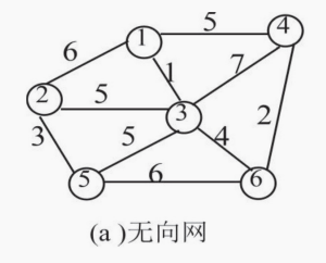
Algorithmic thought process:

Set up 2 data structures:

lowcost[i]: In this example, the array subscript starts from 0, lowcost[i] corresponds to the vertex i+1 in the graph, and records the minimum connecting edge weight from the selected vertex set to the vertex.The edge weights in the graph are all greater than 0, so 0 is used to mark the vertex as having been added to the minimum spanning tree (MST).

visitInfo: indicates the node that has been visited.

1. Initialize with vertex 1 as the starting point, and update lowcost each time a new vertex is added (∞ means that there is currently no edge connecting U to the vertex):

The selected edges and the updated complete array are listed below, corresponding to the subsequent process table.

// 数组各项依次对应顶点 1、2、3、4、5、6
初始化：                   lowcost = [0, 6, 1, 5, ∞, ∞]
选边 (1,3)，加入顶点 3：    lowcost = [0, 5, 0, 5, 5, 4]
选边 (3,6)，加入顶点 6：    lowcost = [0, 5, 0, 2, 5, 0]
选边 (6,4)，加入顶点 4：    lowcost = [0, 5, 0, 0, 5, 0]
选边 (3,2)，加入顶点 2：    lowcost = [0, 0, 0, 0, 3, 0]
选边 (2,5)，加入顶点 5：    lowcost = [0, 0, 0, 0, 0, 0]

The above figure is expressed in a table as follows:

Among them ( ∞ means it doesn’t matter)

	1	2	3	4	5	6
1	∞	6	1	5	∞	∞
2	6	∞	5	∞	3	∞
3	1	5	∞	7	5	4
4	5	∞	7	∞	∞	2
5	∞	3	5	∞	∞	6
6	∞	∞	4	2	6	∞

Example: V={1,2,3,4,5,6}.Taking vertex 1 as the starting point, initialize U={1}, W={2,3,4,5,6}.

The process of implementing Prim's algorithm:

U represents the vertex set that has been added to the spanning tree, and W represents the vertex set that has not been added.At each step, the minimum weight edge connecting U and W is selected, the edge is added to the spanning tree, and the corresponding vertex in W is moved into U.

The bold numbers in U in the table represent the newly added vertices in this step, and ∅ represents the empty set.

Steps	Select edges/weights	U (selected)	W (not selected)
Initialization	—	{1}	{2, 3, 4, 5, 6}
1	(1,3) / 1	{1, 3}	{2, 4, 5, 6}
2	(3,6) / 4	{1, 3, 6}	{2, 4, 5}
3	(6,4) / 2	{1, 3, 6, 4}	{2, 5}
4	(3,2) / 5	{1, 3, 6, 4, 2}	{5}
5	(2,5) / 3	{1, 3, 6, 4, 2, 5}	∅

Finally, 5 edges were selected, with a total weight of 1+4+2+5+3=15.In step 4, you can also select the edge (3,5) with the same weight, and then select (5,2) to get another minimum spanning tree with the same total weight of 15.

2️⃣ Minimum spanning tree algorithm: Kruskal algorithm (kruskal)

The basic idea of Kruskal's algorithm is: Sort all edges in the graph by increasing weight, and select edges in order that will not form a loop with the selected edge.For a connected graph with n vertices, just select n-1 edges.

Time complexity:

The time overhead of Kruskal's algorithm mainly comes from the sorting of edges.Assuming the number of edges is e, when using efficient union-find implementation, the time complexity is usually O(e log e), which is suitable for sparse graphs with a small number of edges.

Algorithm steps:

a. Sort the storage structure of the graph according to the weight from small to large.

b. Initialize and check the set so that each vertex belongs to a set.

c. Check each edge according to the weight value from small to large.If the vertices at both ends belong to the same set, skip the edge; otherwise, proceed to step d.

d. Add the edge to the spanning tree, accumulate weights, and merge the sets of vertices at both ends.For example, the following figure first selects edge (1,3), whose weight is 1.If the array to be merged is a, initially a[1]=1 and a[3]=3 are set, and the two sets can be merged by setting a[1]=3.Repeat the above process until n-1 edges are selected.

【 Note 】 ： Union Find-Graph Connectivity

Kruskal's minimum spanning tree process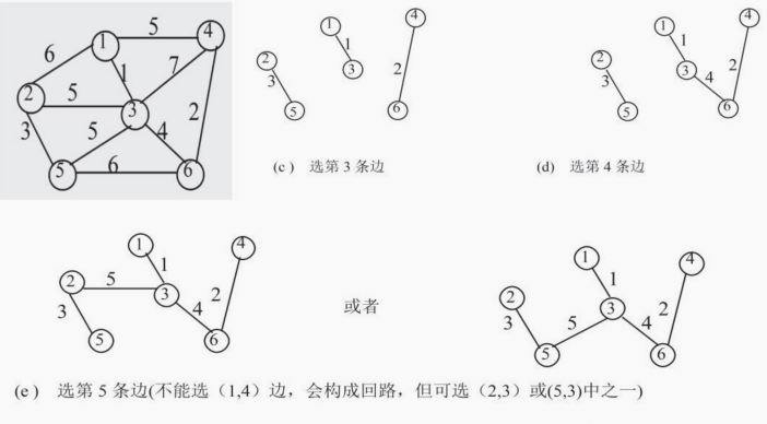

Finally, you can choose (2,3) or (3,5). The weights of both edges are 5, so the minimum spanning tree is not unique and the total weight is 15.

circle avoidance method:

Both Prim's algorithm and Kruskal's algorithm construct a minimum spanning tree by gradually adding edges.Prim selects the minimum weight edge connecting the selected vertex set and the unselected vertex set each time; Kruskal selects edges that will not form a loop in the order of increasing global edge weight. Both algorithms ensure that no loop is formed when adding edges. This construction method is called the loop avoidance method.Prim avoids loops by adding one unselected vertex at a time, while Kruskal can use a union lookup to determine whether a loop is formed.

Circle breaking method:

Starting from the complete connected network, the maximum weight edges in the ring are gradually deleted while maintaining the connectivity of the graph.When n-1 edges remain, a minimum spanning tree is obtained.

Algorithmic Thought:

1. Check each edge from largest to smallest weight.If the edge is in a loop, delete it; if deletion will make the graph disconnected, keep it.
2. Repeat the above process until the number of remaining edges is n-1 and the construction is completed.

👉apply3️⃣:shortest path

There are two ways to discuss the shortest path: The shortest path of a single source point and the shortest path of all pairs of vertices.

Shortest path from a single source: Dijkstra’s algorithm

Definition: The shortest path of a single source point means: given a starting point (single source point) and a directed network G=(V, E), find the shortest path from the source point to other vertices.
Question: How to find the shortest path from a single source point?
Answer: List all the paths from the source point to the end point, and then choose the shortest one.This enumeration method can be implemented by computer, but the efficiency is very low when there are many paths.
Method: After making a lot of observations, Dijkstra first proposed the shortest path algorithm that generates vertices in increasing order of path length, which we call Dijkstra's algorithm.
Algorithmic idea: Dijkstra's algorithm is suitable for graphs with non-negative edge weights.Let V be the set of all vertices in the network, set up and gradually expand a set S to store the vertices whose shortest paths have been found, then the set of vertices V-S whose shortest path has not yet been determined: add the vertices in V-S to S one by one in the order of increasing path length, until the shortest paths of all vertices have been determined, or the remaining vertices are unreachable.Each time, the vertex that has not yet been determined and whose current distance is the smallest is selected, added to S, and the distance of its adjacent vertices is updated.If the remaining vertices are all ∞, the calculation ends and they are unreachable from the source point.

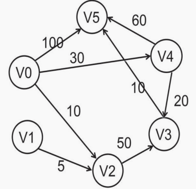
Endpoint	The shortest path from V0 to each end point
	i=1	i=2	i=3	i=4	i=5
V1	∞	∞	∞	∞	∞
V2	10(V0,V2)
V3	∞	60(V0,V2,V3)	50(V0,V4,V3)
V4	30(V0,V4)	30(V0,V4)
V5	100(V0,V5)	100(V0,V5)	90(V0,V4,V5)	60(V0,V4,V3,V5)
VK	V2	V4	V3	V5	None
Path	V0-V2	V0-V4	V0-V4-V3	V0-V4-V3-V5
S	{V0,V2}	{V0,V2,V4}	{V0,V2,V4,V3}	{V0,V2,V4,V3,V5}

Dijkstra's algorithm adopts greedy thinking and gradually determines the shortest path from the source point to each vertex in the order of increasing shortest distance.In the above figure, the shortest distances from V0 to V2, V4, V3, and V5 are 10, 30, 50, and 60 respectively, while V1 is unreachable from V0.After the calculation is completed, you can directly query the shortest distance from the source point to the target vertex.

Shortest path between all pairs of vertices: Floyd's algorithm

The shortest path between all pairs of vertices is: For a given directed network G=(V,E), for any ordered pair of vertices V and W in G (V<>W), find the shortest distance from V to W and the shortest distance from W to V.
Effective method to solve this problem: For graphs with non-negative edge weights, you can perform Dijkstra's algorithm with each vertex as the source point in turn.You can also use Floyd's algorithm to directly calculate the shortest path for all pairs of vertices, with a time complexity of O(n³).

Floyd algorithm idea:

Initialize the distance matrix D with the weight matrix of the graph, where D[i][j] represents the current shortest distance from vertex i to j.Each vertex is used as an intermediate vertex in turn, the distance is compared and updated, and the shortest distance matrix of all vertex pairs is finally obtained.

Floyd-warshall algorithm description:

// floydWarshell
let n = 4;
let arcs = [
    [0, 3, Infinity, 7],
    [8, 0, 2, Infinity],
    [5, Infinity, 0, 1],
    [2, Infinity, Infinity, 0]
]

function floydWarshell() {
    for (let k = 0; k < n; k++) {
        for (let i = 0; i < n; i++) {
            for (let j = 0; j < n; j++) {
                arcs[i][j] = min(arcs[i][j], arcs[i][k] + arcs[k][j])
            }
        }
    }
}

function min(num1, num2) {
    return num1 < num2 ? num1 : num2;
}

floydWarshell();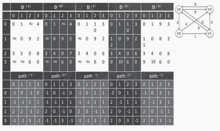

The figure above uses another set of data to demonstrate the process of Floyd's algorithm updating the distance matrix and path records round by round.In each round, a vertex k is selected as the intermediate vertex, and D[i][j] is compared with D[i][k] + D[k][j]. If the path through k is shorter, the distance and corresponding path record are updated.In the graph, vertices 0, 1, 2, and 3 are used as intermediate vertices to complete the update.

👉Apply4️⃣:topological sorting

Usually we regard planning, construction process, production process, etc. as a project. A large project is often divided into many smaller sub-projects. These sub-projects are called activities. When these activities are completed, the entire project is completed.

AOV network introduction

In this directed graph, the vertices represent activities, and the directed edges represent the priority relationships of activities. This directed graph is called a network with vertices representing activities (Activity On Vertex), or AOV network for short.
In the AOV network, the <i,j> directed edge indicates that activity i should start before activity j, that is, activity i must be completed before activity j can start, and i is called the direct predecessor of j, and j is the direct successor of i.This relationship between precursor and successor is transitive. In addition, any activity i cannot use itself as its predecessor or successor. This is called anti-reflexivity.From the perspective of the transitivity and anti-reflexivity of the predecessor and successor, directed loops (or directed loops) cannot appear in the AOV network. For engineering, it will be impossible: for program flow, there will be an infinite loop.

Steps of topological sorting:

1. Select a vertex with indegree 0 in the AOV network and output
2. Delete this vertex and all directed edges emanating from this vertex in the AOV network
3. Repeat steps 1 and 2 until all vertices in the AOV network are output or there are no vertices with an in-degree of 0 in the network.

👉application5️⃣:critical path

If the vertices of a weighted directed graph represent events or project progress status, arcs are used to represent activities, and the weights on the arcs represent the time required to complete the activity, then such a weighted directed graph is called an AOE network (Activity On Edge Network).

1. Only after the event represented by a vertex occurs, the activities represented by the directed edges starting from the vertex can begin.
2. The event represented by the vertex can only occur when the activities represented by the directed edges entering a vertex have ended.

Critical Path (critical path): The longest path from a source to a sink (end vertex) in an AOE network.Activities on the critical path are critical activities.

Summary

1: Prim is an algorithm for calculating the minimum spanning tree. For example, how to build roads for N villages with the least cost.

Dijkstra is an algorithm for calculating the shortest path, such as the distance from village A to any other village.

2: Prim algorithm updates the minimum connecting edge weight from the selected vertex set to each unselected vertex;

Dijkstra's algorithm updates the current shortest distance from the source point to each undetermined vertex;

3. Prim is better than Kruskal in dense graphs and worse than Kruskal in sparse graphs.

Graph storage and traversal

Shortest path problem

floyd-warshell